Dynamical Systems

Lesson

Lyapunov Exponent

The Lyapunov exponent, measures how quickly an infinitesimally small distance between two initially close states grows over time.

$| F(x_0 + \epsilon, t) - F(x_0, t) | \sim \epsilon e^{\lambda t} \\$

The left hand side is the distance between two initially close states after steps, and the right hand side is the assumption that the distance grows exponentially over time. The Lyapunov exponent which is measured for long period of time corresponds to the exponent . The stability of the system is given by the sign of . If : means that s small distance grow with time, this corresponds to the stretching mechanism. 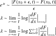And if : small distance do not grow indefinitely.The expression of is obtained by doing some mathematical derivation, as follows:

$e^{\lambda t} \sim \frac{| F(x_0 + \epsilon, t) - F(x_0, t) | }{\epsilon }\\ \quad\\ \lambda \sim \lim \limits_{r \rightarrow \infty}\frac{1}{t} \log \Big\vert \frac{dF}{dx} \Big\vert_{x = x_0} \Big\vert \\ \quad\\ \lambda \sim \lim \limits_{r \rightarrow \infty}\frac{1}{t} \log \sum_{i=0}^{t-1} \Big\vert \frac{dF}{dx} \Big\vert_{x = x_i} \Big\vert$

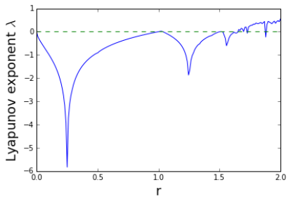
Taking the example of non-linear equation described above, we can calculate the Lyapunov exponent for different values of :

$\frac{dx}{dt} = r-x^2$

We can observe that the system becomes chaotic from a certain value of . The reader can play with different values of by using the following code source.

Visual output of the following code, showing the Lyapunov exponent of the above equation

@author: yacine.mezemate
"""
import numpy as np
import matplotlib.pyplot as plt
global x0, r
x0 = 0 # Initial condition
r = np.linspace(0,2,200) # Parameter r
# Differential equation
def F(x0,r):    
    x = np.zeros((100,200))
    
    for j in range(0,200):
        
        x[0,j] = x0 
        for i in range(0,99):
            x[i+1,j] = x[i,j] + r[j] - x[i,j]**2 
    return x            
# Derivative
def dF(x):
    dy = np.log(abs(1-x*2))
    return dy
# Lyapunov exponent    
def Lyapunov(dy):
    Lambda = np.mean(dy, axis =0)
    return Lambda
    
# main    
y = F(x0,r)
dy = dF(y)
lam = Lyapunov(dy)
# PLot
plt.plot(r,lam)
plt.plot([0,2], [0,0], "--")
plt.xlabel("r", fontsize =18)
plt.ylabel("Lyapunov exponent $\lambda$", fontsize =18)

@author: yacine.mezemate
"""
import numpy as np
import matplotlib.pyplot as plt

global x0, r

x0 = 0 # Initial condition
r = np.linspace(0,2,200) # Parameter r

# Differential equation
def F(x0,r):    
    x = np.zeros((100,200))
    
    for j in range(0,200):
        
        x[0,j] = x0 

        for i in range(0,99):
            x[i+1,j] = x[i,j] + r[j] - x[i,j]**2 
    return x            

# Derivative
def dF(x):
    dy = np.log(abs(1-x*2))
    return dy

# Lyapunov exponent    
def Lyapunov(dy):
    Lambda = np.mean(dy, axis =0)
    return Lambda
    
# main    
y = F(x0,r)
dy = dF(y)
lam = Lyapunov(dy)

# PLot
plt.plot(r,lam)
plt.plot([0,2], [0,0], "--")
plt.xlabel("r", fontsize =18)
plt.ylabel("Lyapunov exponent $\lambda$", fontsize =18)

Homepage