Multi-Scale Simulation

Lesson

Introduction
Random dynamical system
Brownian motion
Multifractal simulation
Effect of variation of UM parameters on simulation
To go further
Exercises
- Quiz: Continuous cascade
- Quiz: Non conservative field
Conclusion

Non conservative field

In the previous exercise we play with the different step to construct a multifracta continuous field using a Lévy generator. These constructions are not valid for a non conservative quantities such as the velocity field or passive scalar. In this exercise we will see how to construct a non conservative field using the Fractional Integrated Field technique presented in this lecture.

Question

Starting with the given programs (previous exercise) generated a continuous field.

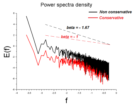
Plot the power spectra density of the generated field.

We have seen in the previous lecture that the slope of PDS is related to the Hurst exponent (non-conservativeness parameter) by the following relation:

$H = \frac{\beta -1 + K(2)}{2}$

Assuming the intermittency correction is null calculate the parameter using the PDS slope.

Generate a non conservative field with , by using the following program with previous programs.

// Fractional Integration 
function [Field]=FracIntegration(flux, lambda, a, H)
    flux = flux.^a;
    F = fft(flux);
    N = lambda/2 +1;
    n = 1:N;
    F(1:N) = F(1:N).*(n.^(-H));
    F(N+1:lambda) = real(F(lambda/2:-1:2)) -%i*imag(F(lambda/2:-1:2));
    
    Field = ifft(F);
    Field = real(Field(1,1:lambda));
    
endfunction

// Fractional Integration 
function [Field]=FracIntegration(flux, lambda, a, H)
    flux = flux.^a;
    F = fft(flux);
    N = lambda/2 +1;
    n = 1:N;
    F(1:N) = F(1:N).*(n.^(-H));
    F(N+1:lambda) = real(F(lambda/2:-1:2)) -%i*imag(F(lambda/2:-1:2));
    
    Field = ifft(F);
    Field = real(Field(1,1:lambda));
    
endfunction

Plot and compared the PDS of the obtained field with previous generated field.

Calculate the slope spectra of non conservative field using the value of according to the previous relation.

Hint

Power spectra intermittency correction : .

Solution

// Fractional Integration 
function [Field]=FracIntegration(flux, lambda, a, H)
    flux = flux.^a;
    F = fft(flux);
    N = lambda/2 +1;
    n = 1:N;
    F(1:N) = F(1:N).*(n.^(-H));
    F(N+1:lambda) = real(F(lambda/2:-1:2)) -%i*imag(F(lambda/2:-1:2));
    
    Field = ifft(F);
    Field = real(Field(1,1:lambda));
    
endfunction

// Fractional Integration 
function [Field]=FracIntegration(flux, lambda, a, H)
    flux = flux.^a;
    F = fft(flux);
    N = lambda/2 +1;
    n = 1:N;
    F(1:N) = F(1:N).*(n.^(-H));
    F(N+1:lambda) = real(F(lambda/2:-1:2)) -%i*imag(F(lambda/2:-1:2));
    
    Field = ifft(F);
    Field = real(Field(1,1:lambda));
    
endfunction

clear;
clc;
exec("Levy.sce");
exec("FracIntegration.sce");
exec("ColorFunc.sce");
exec("Continuous.sce");
exec("Slope.sce");
// Universal multifractal parameters
alpha = 1.7;
C1 = 0.5;
lambda = 2^12;
// Continuous simulation
Sim = Continuous(alpha,C1,lambda);
// Calculate the spectrum
tamp1 = abs(fft(Sim));
E1 = tamp1.*tamp1;
E1 = E1(1:length(E1)*0.5)
// Fractional integration
a = 1/3;
H =1/3;
Field = FracIntegration(Sim, lambda, a, H);
// Calculate the spectrum
tamp = abs(fft(Field));
E = tamp.*tamp;
x = (1:length(E)*0.5)/length(E);
E = E(1:length(E)*0.5)
// Spectra slope estimation
break_frequence =[0.5 0.001];
Scalingrange=[1 length(E)*break_frequence(2);length(E)*break_frequence(2) length(E)*break_frequence(1)]
s = Slope(E,Scalingrange);
s1 = Slope(E1,Scalingrange); 
    
//Plots
plot2d(log10(x), log10(E1),5)
plot2d(log10(x), log10(E))

clear;
clc;

exec("Levy.sce");
exec("FracIntegration.sce");
exec("ColorFunc.sce");
exec("Continuous.sce");
exec("Slope.sce");

// Universal multifractal parameters
alpha = 1.7;
C1 = 0.5;
lambda = 2^12;

// Continuous simulation
Sim = Continuous(alpha,C1,lambda);

// Calculate the spectrum
tamp1 = abs(fft(Sim));
E1 = tamp1.*tamp1;
E1 = E1(1:length(E1)*0.5)

// Fractional integration
a = 1/3;
H =1/3;
Field = FracIntegration(Sim, lambda, a, H);

// Calculate the spectrum
tamp = abs(fft(Field));
E = tamp.*tamp;
x = (1:length(E)*0.5)/length(E);
E = E(1:length(E)*0.5)

// Spectra slope estimation
break_frequence =[0.5 0.001];
Scalingrange=[1 length(E)*break_frequence(2);length(E)*break_frequence(2) length(E)*break_frequence(1)]

s = Slope(E,Scalingrange);
s1 = Slope(E1,Scalingrange); 
    
//Plots
plot2d(log10(x), log10(E1),5)
plot2d(log10(x), log10(E))

Power spectra density for conservative and non-conservative field field

Homepage