
Brownian Motion equation
The Brownian Motion, named in honor of the botanist Robert Brown, describes the motion of particle subjected to an infinity of shocks in very short time, and its and its trajectories are irregular. They have the following proprieties:
The trajectory of the particle at the time prior of
 does not acts on the future trajectories. This propriety is called a Markov propriety.
The particles move continuously in space.
The law of the position of the particle between two instants
and
 depends only on
 . The increases are then stationary.
If
 denotes the position of the particle at the time
, and due to the previous proprieties it is easy to show that
follows a normal distribution , with zero mean and a variance
.
denotes the position of the particle at the time
, and due to the previous proprieties it is easy to show that
follows a normal distribution , with zero mean and a variance
.
For a short time scale, the particles are pushed in some direction, this implies that the average position at the time
 knowing the position
is given by
knowing the position
is given by
 for a vector
 , which can also depends on
. We can write :
, which can also depends on
. We can write :
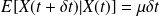
Where
 is a normal Gaussian centered covariance identity. It is easy to check that:
![E[X(t + \delta t) | X(t)] = \mu \delta t\\ \quad \\ And \\ \quad\\ E[ (X(t + \delta t)- E[X(t + \delta t) | X(t)] )^2] = \sigma (X(t)) \sigma (X(t))^T \delta t](../res/eq6.png)
Where
 is a matrix-valued function (which is not necessarily a square matrix), and
a vector-valued function.
is a matrix-valued function (which is not necessarily a square matrix), and
a vector-valued function.


