
Saddle-Node Bifurcation
We have introduced above the Saddle-Node bifurcation without naming it. This bifurcation is associated to the differential equation:
 , where
 and
and
 are the control parameters. For
 we are speaking about subcritical bifurcation. Lets
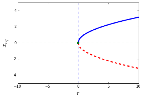
 , the equilibrium points are easy to determine and they are immediately obtained :
 , this means that the equilibrium point exist only for
 . We can summarize the result in the following table:
Equilibrium point |
|
|
| doesn't exist | stable |
| doesn't exist | unstable |


The visualization can be done in the bifurcation diagram:
1
from pylab import *
2
def xeq1(mu):
3
return sqrt(mu)
4
def xeq2(mu):
5
return -sqrt(mu)
6
domain = linspace(0, 10)
7
plot(domain, xeq1(domain), 'b-', linewidth = 3)
8
plot(domain, xeq2(domain), 'r--', linewidth = 3)
9
plot([0], [0], 'go')
10
plot([0,0],[-5,5], "--")
11
plot([-10,10],[0,0], "--")
12
axis([-10, 10, -5, 5])
13
xlabel('$r$', fontsize = 18)
14
ylabel('$x_{eq}$', fontsize = 18)
15
show()16
For
 we are speaking about super-critical bifurcation.


