
Linearization
The simplest description of the phenomena in question consists to take into account only the preponderant terms of the magnitudes in play and do not take into account those of lesser importance, which are considered to be corrective terms. In fact, this method called linearization, allowed us to recognize many elements invariant and great regularity in natural phenomena. Especially in classical physics, linearization has enabled us to deal with various phenomena with a high degree of approximation, although many other, fundamental problems remain unresolved. The idea is simply that, as the terms that have been ignored by linearized equations were small, the difference between the solutions of the linearized equation and those of the nonlinear equation supposed "real", but unknown, should be low as well; However, this is not always the case.
We will give a quick example of the linearization. To that, lets a given non-linear equation, represented in the below figure.
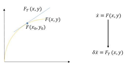
The first step a linearization is to calculate the fixed point for which the derivative is equal to zero. The second step, is to rewrite the equation of the system for the perturbed fixed point
 . The linearization consists of using the Taylor expansion of the non-linear term. Ignoring the high order of Taylor series expansion, we will obtain the linear differential equation.
Linearization of a nonlinear differential or difference equation about a given trajectory (in particular an equilibrium state) yields a linear system which, in general, will be time-varying. Since stability is a local property one might expect that the linearization provides sufficient information to determine whether or not the trajectory is stable. This is the idea behind an approach adopted by Liapunov which is now known as Liapunov's indirect method.


