Governing equations
Heat transfer
The challenge in this practical is to calculate the heat flux across the bottom of the ocean thermocline by solving the diffusion equation in the vertical.
Specifications of the ocean thermocline
Typically the ocean is stably strati ed and its density increases very slowly with depth. A mixed layer exists in the top 10 to 100m of the ocean due mainly to mechanical stirring by turbulence associated with wind stresses. Between the mixed layer and the deep ocean there can be a strong temperature gradient called the thermocline. In this practical, assume that the mixed layer is very shallow so that fluxes from the atmosphere feed directly into the thermocline. Take the thermocline to have a fixed depth of 200m with uniform thermal diffusivity
 and density
 . The abyssal ocean below is at a fixed temperature of

Initial and boundary conditions
Initially, the temperature is well-mixed across the top 20m with a temperature of
 . Temperature decreases linearly from 20m to the abyssal temperature (
 ) at 200m depth. Assume that there are no fuxes across the top and bottom boundaries of the thermocline.
Question
Write a program to solve this model.
Question
Use a time-step of 3,600s. Conduct a 5-day experiment and investigate the change in temperature profile with time by plotting temperature versus depth at least once per day.
Question
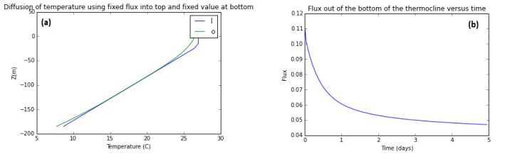
Now implement more realistic boundary conditions. Assume that there is a constant heat flux into the ocean surface at rate
 and the temperature of the bottom boundary is fixed and equal to the abyssal temperature. In this case the flux across the bottom boundary is not specified. Run the model for 1,000 days
# -*- coding: utf-8 -*-
"""
Created on Tue May 10 10:08:27 2016
Program to model the diffusion of temperature
@author: yacine.mezemate
"""
import numpy as np
import matplotlib.pyplot as plt
#define the physical constants
dcoeff=1.0e-3 # diffusion coefficient (m^2/s)
depth=200. # thermocline depth (m)
density=1000 # density (kg m^-3)
tint=5*86400. # total run length (secs)
fluxtop=0.01 # flux into thermocline (kg m^-2 K s^-1)
# define the numerical constants
nlev=20 # Number of model levels
dz=depth/nlev # Spacing between model levels
dt=3600.0 #time-step (unit=secs)
nsteps=tint/dt #number of time-steps
dfac=dcoeff*dt/(dz*dz) #factor used in numerical scheme
#declare arrays to store the results
z= np.zeros(nlev)
tempnew=np.zeros(nlev) # new value of temperature (in each layer)
temp=np.zeros(nlev) # current temperature
tinit=np.zeros(nlev) # initial temperature
time=np.zeros(nsteps) #array of time-points
fluxbot=np.zeros(nsteps) # flux through bottom of thermocline
# fill in the initial values of the arrays
t=0.0;
tair=27.0;
tabyss=7.0;
zmix=20 # depth of the well-mixed part of initial profile
# specify initial temperature profile
for i in range(0,nlev):
z[i] = (i -0.5)*dz
tinit[i]=tabyss+(tair-tabyss)*(z[i]-depth)/(zmix-depth)
if (tinit[i] > tair):
tinit[i] = tair
temp = tinit
for n in range(0,int(nsteps)):
#Find new temperature in the top layer (applying flux BCs)
tempnew[0]=temp[0]+dfac*(temp[1]-temp[0])+fluxtop*dt/(density*dz)
#Find new temperature for all interior layers
for j in range(1,nlev-1):
tempnew[j]=temp[j]+dfac*(temp[j+1]-2*temp[j]+temp[j-1])
#Find new temperature in the bottom layer (applying fixed value BCs)
tempnew[nlev-1]=temp[nlev-1]+dfac*(2*tabyss-3*temp[nlev-1]+temp[nlev-2])
# Find flux through bottom of the thermocline
time[n]=t/86400
fluxbot[n]=-density*dcoeff*(temp[nlev-1]-tabyss)/(z[nlev-1]-depth)
t=t+dt #Find the new time-point
temp=tempnew #Copy new temperatures into temp array before next step
plt.figure(1)
plt.plot(tinit,-z, label='Initial')
plt.plot(tempnew,-z, label='1000 days')
plt.legend('loc= down left')plt.title("Diffusion of temperature using fixed flux into top and fixed value at bottom")plt.xlabel("Temperature (C)")plt.ylabel("Z(m)")plt.show()
plt.figure(2)
plt.plot(time,fluxbot)
plt.title("Flux out of the bottom of the thermocline versus time")plt.xlabel("Time (days)")plt.ylabel("Flux")plt.show()