Data analysis
Data analysis
As shown in this lecture, the spectral analysis is used to identify the involved process, and also to chuck the propriety of scale invariance. In this exercise we use velocity data from JHU wind tunnel[1] to characterize the process.
Question
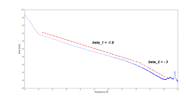
Unzip the data file and plot the corresponding PSD, divide the data sample into sub-samples of length 4096 points and perform the Fourier transform on each.
Compute the average spectrum and plot
 , where
 is the frequency.
Check if there is scaling break and evaluate the spectral slope
 on range if scale.
Solution
1
"""2
@author: yacine.mezemate3
"""4
import numpy as np
5
import scipy as sp
6
import matplotlib.pylab as plt
7
8
#Load data9
data = np.loadtxt('data.txt')
10
11
#Define length data12
LenMax = data.shape[0]
13
SampleLenght = sp.power(2,12)
14
Nb = LenMax/SampleLenght
15
16
#Memory allocation17
FMax=np.floor(SampleLenght/2)
18
f = sp.arange(1,FMax+1,1)
19
E = sp.zeros((FMax,Nb))
20
21
#Calculate the PSD for each sub-sample22
for j in range(Nb-1):
23
24
DataSample = data[SampleLenght*j:(j+1)*SampleLenght]
25
Buffer = np.absolute(np.fft.fft(DataSample))
26
E[:,j]=Buffer[0:FMax]*Buffer[0:FMax]
27
28
# Calculate the average PSD 29
E_m = E.mean(1)
30
31
#Plot the average PSD32
plt.loglog(f,E_m, basex =2)
33
plt.xlabel("Frequency [f]", fontsize = 18)
34
plt.ylabel("PSD [E(f)]", fontsize = 18)
35
36
# Calculate the slope for different range of scale37
scale1 = 0
38
scale2 = 8
39
scale3 = []40
41
if scale3 == []:
42
rng = [sp.power(2,scale1),sp.power(2,scale2)]
43
else: 44
rng = [sp.power(2,scale1),sp.power(2,scale2), sp.power(2,scale3)]
45
46
rngLen = len(rng)
47
48
if rngLen ==2:
49
Fmin = rng[0]
50
Fmax = rng[1]
51
slope = sp.polyfit(np.log2(f[Fmin:Fmax]),np.log2(E_m[Fmin:Fmax]),1)
52
reg_lin=sp.poly1d(slope)
53
beta1 = slope[0]
54
55
print("beta 1 = "+ str(round(beta1,2)))
56
57
elif rngLen == 3:
58
#beta 1 59
Fmin = rng[0]
60
Fmax = rng[1]
61
slope = sp.polyfit(np.log2(f[Fmin:Fmax]),np.log2(E_m[Fmin:Fmax]),1)
62
reg_lin=sp.poly1d(slope)
63
beta1 = slope[0]
64
#beta 265
Fmin = rng[1]
66
Fmax = rng[2]
67
slope = sp.polyfit(np.log2(f[Fmin:Fmax]),np.log2(E_m[Fmin:Fmax]),1)
68
reg_lin=sp.poly1d(slope)
69
beta2 = slope[0]
70
71
print("beta 1 = " + str(round(beta1,2)), "beta 2 = " + str(round(beta2,2)))
72


