Spectral Analysis

Lesson

Introduction
Some definitions
- Definition
- Some applications
- Spectral analysis is based on Fast Fourier transform FFT
- Discrete Fourier transform DFT
Power spectral density (PSD)
Scaling analysis
Identification of some processes
Exercises
To go further
Conclusion

Discrete Fourier transform DFT

If or is known analytically or numerically, the above integrals can be evaluated using the integration techniques. In practice, the signal is measured at just a finite number of times , and these are what we must use to approximate the transform. The resultant discrete Fourier transform is an approximation both because the signal is not known for all times and because we integrate numerically. The DFT algorithm results from evaluating the integral not from and but rather from time to time over which the signal is measured, and by using

the trapezoid rule for the integration:

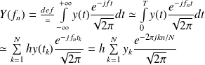
$Y(f_n) = {def\over{=}} \int \limits_{- \infty}^{+ \infty} y(t) \frac{e^{-jft}}{\sqrt{2 \pi}} dt \simeq \int \limits_{0}^{T} y(t) \frac{e^{-jf_nt}}{\sqrt{2 \pi}} dt \\ \quad \\ \simeq \sum \limits_{k=1}^{N} h y(t_k) \frac{e^{-jf_nt_k}}{\sqrt{2 \pi}} = h \sum \limits_{k=1}^{N} y_k \frac{e^{-2 \pi jkn /N}}{\sqrt{2 \pi}}$

To keep the final notation more symmetric, the step size is factored from the transform and a discrete function is defined:

$Y(f_n) = {def\over{=}}\frac{1}{h} Y(f_n) = \sum \limits_{k=1}^{N} y_k \frac{e^{-2 \pi jkn /N}}{\sqrt{2 \pi}}$

With this same care in accounting, and with , we invert the 's:

$y(t) = {def\over{=}} \int \limits_{- \infty}^{+ \infty} Y(f) \frac{e^{jft}}{\sqrt{2 \pi}} df \simeq \sum \limits_{n=1}^{N} \frac{2 \pi}{Nh} \frac{e^{jf_nt}}{\sqrt{2 \pi}} Y(f_n)$

Homepage