β-model
As we have seen in lesson Fractals, we can characterizes the occurrence of the rainfall by its fractal dimension Df. The main goal of this exercise is to reproduce the pattern of rainfall occurrence according to some given parameter (co-dimension).
Question
1 - According to cascade principle : determine the possible states after n steps.
2 - Play with different values of C, and interpret the obtained result
3 - For the same value of C run the simulation different times and discuss the obtained field.
4 - Use the given python code to generate different field in 1D/2D.
1 - After n steps of cascade the state of the field can be expressed as follows:

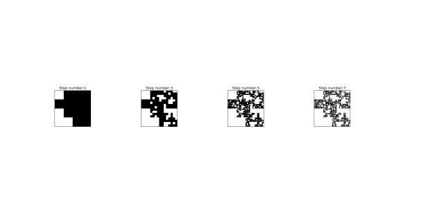
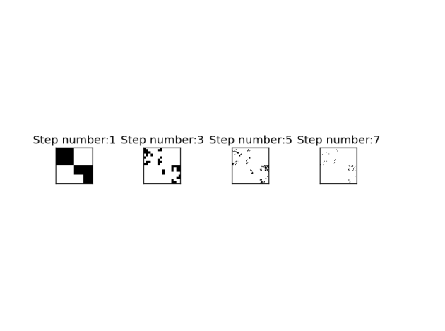
2 - Decreasing the value of the co-dimension
 the obtained field is more homogenous (less intermittent), and increasing the value of
 this yields to a field which is more intermittent (see figures).
3 - For the same value of
 and running the simulation several times, the obtained field is not the same visually, but the they are similar statistically.
# -*- coding: utf-8 -*-"""@author: yacine.mezemate"""import scipy as sp
from scipy.stats import uniform
import matplotlib.pyplot as plt
def BetaModel(Lambda, C, nsteps, dimension):
if dimension == 1:
DataInit = sp.ones(1)
for t in range(nsteps):
length = sp.power(Lambda,t+1)
DataBuff = sp.ones((length,1))
for k in range(0,length):
index = sp.floor((k+2)/Lambda) -1
mu = uniform.rvs()
if mu <= sp.power(Lambda,-C):
DataBuff[k] = DataInit[index]*sp.power(Lambda,C)
else:DataBuff[k] = 0
DataInit = DataBuff
if dimension == 2:
DataInit = sp.ones((1,1))
for t in range (nsteps):
length = sp.power(Lambda,t+1)
DataBuff = sp.ones((length,length))
for k in range(0,length):
for l in range(0,length):
indexI = sp.floor((k+2)/Lambda)-1
indexJ = sp.floor((l+2)/Lambda)-1
mu = uniform.rvs()
if mu <= sp.power(Lambda,-C):
DataBuff[k,l] = DataInit[indexI,indexJ]*sp.power(Lambda,C)
else:DataBuff[k,l] = 0
if t % 2:
plt.subplot(1,nsteps,t)
plt.imshow(DataBuff,interpolation='nearest',cmap='Greys')
plt.title("Step number:" + str(t))
frame = plt.gca()
frame.axes.get_xaxis().set_ticks([])
frame.axes.get_yaxis().set_ticks([])
plt.show()
DataInit = DataBuff
return DataInit
############################################################################################################ Parameters ######################################Lambda = 2
C = 0.8
nsteps = 8
dimension = 1
############################# Cascade ######################################### DataSim = BetaModel(Lambda, C, nsteps,2)


