
UM estimation
The multifractal analysis is a very powerful method to characterize the variability of the environmental field. It allows us to calculate (if it is possible) the high order moments which are used to estimate the PDF of the field. In this exercise we use the multifractal analysis to characterize the variability of a temperature time series.
Question
Use the given script (using the TM method) to estimate the
 for
for
 ranging from 0 to 6
Calculate the UM parameters using the first and the second derivative of
Compare the theoretical
with the empirical one
Use the DTM to estimate the UM parameter.
Use the definition of the maximum observable singularity to estimate the
 .
.
Hint
 ,
,

Solution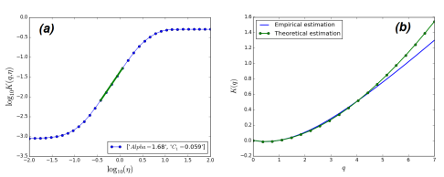
1
2
"""3
@author: yacine.mezemate4
"""5
import scipy as sp
6
import numpy as np
7
import matplotlib.pylab as plt
8
import math
9
10
#***************** Analysis function***********************11
def Analysis(*args):
12
13
# args[0] = data, args[1] = q14
# args[2] = eta, args[3] = AnalysisType15
flux = args[0]
16
Lmax = flux.shape[0]
17
Nmax = math.log(Lmax,2)
18
19
# Lambda20
l = sp.zeros((Nmax+1))
21
for k in range(int(Nmax)+1):
22
l[k]=sp.power(2,k)
23
#Order24
q = args[1]
25
Nbq = q.shape[0]
26
27
#########################Evaluate Moments#########################28
if args[3]==1: # Trace Moment Analysis
29
30
Moments = np.zeros((Nmax+1,Nbq))
31
32
for j in range(Nbq):
33
Moments[Nmax,j] = np.mean(np.power(flux,q[j]))
34
35
for i in range(int(Nmax-1),-1,-1):
36
37
elem = flux.shape[0]
38
flux = ( flux[0:elem:2] + flux[1:elem+1:2] ) /2
39
40
for n in range(Nbq):
41
Moments[i,n] = np.mean(np.power( flux,q[n] ) )
42
43
#plt.figure(0)44
#plt.loglog(l,Moments)45
46
##############################################################47
48
###########################EvaluateK(q)####################### 49
Kq = np.zeros(Nbq)
50
x = sp.log(l)
51
for n in range(Nbq):
52
y = sp.log(Moments[:,n])
53
slop = sp.polyfit(x,y,1)
54
Kq[n] = slop[0]
55
56
plt.figure(1)
57
plt.plot(q,Kq, lw=2, label='Empirical estimation')
58
plt.xlabel("$q$", fontsize =18)
59
plt.ylabel("$K(q)$", fontsize =18)
60
##############################################################61
62
print("Successful TM analysis")
63
64
elif args[3] == 2: # Double Trace Moment Analysis
65
66
#eta values67
LogEta = args[2]
68
eta = np.power(10, LogEta)
69
NbEta = eta.shape[0]
70
71
#Memory allocation72
Moments = sp.zeros((Nmax+1,Nbq,NbEta))
73
KqEta = sp.zeros((Nbq,NbEta))
74
75
##############################################################76
for i in range(NbEta):
77
78
FluxEta = sp.power(flux,eta[i])
79
80
for j in range(Nbq):
81
Moments[Nmax,j,i] = np.mean(np.power(FluxEta,q[j]))
82
83
for k in range(int(Nmax-1),-1,-1):
84
elem = FluxEta.shape[0]
85
FluxEta = ( FluxEta[0:elem:2] + FluxEta[1:elem+1:2] ) /2
86
87
for j in range(Nbq):
88
Moments[k,j,i] = np.mean(np.power(FluxEta,q[j]))
89
90
##############################################################91
92
#########################Evaluate K(q,eta)####################93
x = sp.log(l)
94
95
for j in range(Nbq):
96
97
for i in range(NbEta):
98
99
y = sp.log(Moments[:,j,i])
100
slop = sp.polyfit(x,y,1)
101
KqEta[j,i] = slop[0]
102
103
Alpha = np.zeros((Nbq,))
104
C1 = np.zeros((Nbq,))
105
106
for j in range(Nbq):
107
AlphaTemp = np.zeros((NbEta,))
108
xEta = np.log10(eta)
109
yEta = np.log10(KqEta[j,:])
110
111
for i in range(15,NbEta-4):
112
sl=sp.polyfit(xEta[i-2:i+3],yEta[i-2:i+3],1)
113
AlphaTemp[i]=sl[0]
114
115
indx=np.argmax(AlphaTemp)
116
a = sp.polyfit(xEta[indx-2:indx+3],yEta[indx-2:indx+3],1)
117
118
Alpha[j]=a[0]
119
C1[j]=np.power(10,a[1])*(a[0]-1)/(q[j]**a[0]-q[j])
120
121
plt.figure(2)
122
plt.plot(xEta,yEta, marker='o', label=['$Alpha =$'+ str(round(Alpha[j],2)),
123
'$C_1 = $' +str(round(C1[j],3)) ] )
124
125
plt.xlabel(r'$\log_{10}(\eta)$',fontsize=20,color='k')
126
plt.ylabel(r'$\log_{10}\mathit{K}(\mathit{q},\eta)$',fontsize=20,color='k')
127
lin=sp.poly1d(a)
128
plt.plot([xEta[indx-2],xEta[indx+2]],[lin(xEta[indx-2]),lin(xEta[indx+2])]
129
,lw=4)
130
plt.legend(loc ='lower right')
131
132
print("Successful DTM analysis")
133
return KqEta, Alpha, C1, Moments
134
135
else:136
print("No Analysis corresponding to the choosed number")
137
#**********************************************************138
def KqTheo(Alpha,C1,q):
139
140
kqTh=np.zeros(q.shape)
141
142
if Alpha == 1:
143
for j in range(q.shape[0]):
144
kqTh[j]=C1*q[j]*np.log(q[j])
145
else:146
for j in range(q.shape[0]):
147
kqTh[j]=C1*(q[j]**Alpha-q[j])/(Alpha-1)
148
149
return kqTh
150
151
#**********************************************************152
#=========================================================153
# Solution154
#========================================================= 155
#*********************** Main *****************************156
data = np.loadtxt('data.txt')
157
l = np.power(2,12)
158
flux = np.abs(np.diff(data[0:l+1]))
159
160
#DTM parameter161
E = np.linspace(-2, 2, 34)
162
q = np.linspace(1.5,1.5,1)
163
Kemp, alph, c, m = Analysis(flux,q,E,2)
164
165
#TM parameter166
q = np.linspace(0,7,20)
167
Analysis(flux,q,E,1)
168
169
K = KqTheo(1.67,0.055,q)
170
171
qs = (1/c)**(1/alph)
172
173
print('qs= '+str(qs))
174
175
plt.figure(1)
176
plt.plot(q,K, marker='o', lw=2, label= 'Theoretical estimation')
177
plt.legend(loc ='upper left')
178


